Graph 🌺

Components of a Graph

• Vertices*/ˈvɜːrtɪsiː/*: Vertices are the fundamental units of the graph. Sometimes, vertices are also known as vertex or nodes. Every node/vertex can be labeled or unlabelled.
• Edges: Edges are drawn or used to connect two nodes of the graph. It can be ordered pair of nodes in a directed graph. Edges can connect any two nodes in any possible way. There are no rules. Sometimes, edges are also known as arcs. Every edge can be labeled/unlabelled.

The graph is denoted by G(V, E).

Types Of Graph

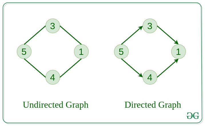
Undirected Graph

• cannot have self loop

A graph in which edges do not have any direction. That is the nodes are unordered pairs in the definition of every edge.

Directed Graph

• self loops allowed

A graph in which edge has direction. That is the nodes are ordered pairs in the definition of every edge.

Weighted Graph

• A graph in which the edges are already specified with suitable weight is known as a weighted graph.
• Weighted graphs can be further classified as directed weighted graphs and undirected weighted graphs.

Dense Graph:

A dense graph is a graph in which there is a large number of edges. Typically in a dense graph, the number of edges is close to the maximum number of edges.

• the maximum edges for a tree: E ≈ V^2. (consider self loops)

Sparse Graph:

A sparse graph is a graph in which there is a small number of edges. In this case the number of edges is considerably less than the maximum number of edges.

the graph which is least dense is actually a tree.

• the minimum edges for a tree: E = V -1. E << V^2

Adjacency

Adjacency relationship is:

• Symmetric if G is undirected.
• Not necessarily so if G is directed.

Here are the norms of adjacency −

• In a graph, two vertices are said to be adjacent, if there is an edge between the two vertices. Here, the adjacency of vertices is maintained by the single edge that is connecting those two vertices.
• In a graph, two edges are said to be adjacent, if there is a common vertex between the two edges. Here, the adjacency of edges is maintained by the single vertex that is connecting two edges.

**Example **

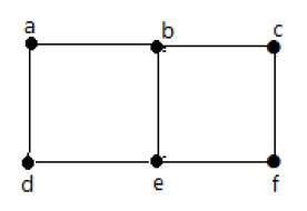
In the above graph −

• ‘a’ and ‘b’ are the adjacent vertices, as there is a common edge ‘ab’ between them.
• ‘a’ and ‘d’ are the adjacent vertices, as there is a common edge ‘ad’ between them.
• ab’ and ‘be’ are the adjacent edges, as there is a common vertex ‘b’ between them.
• be’ and ‘de’ are the adjacent edges, as there is a common vertex ‘e’ between them.

Connected:

if G is connected:

there is a path between every pair of vertices.

From every node you can get to every other node.

Prim’s Algorithm:

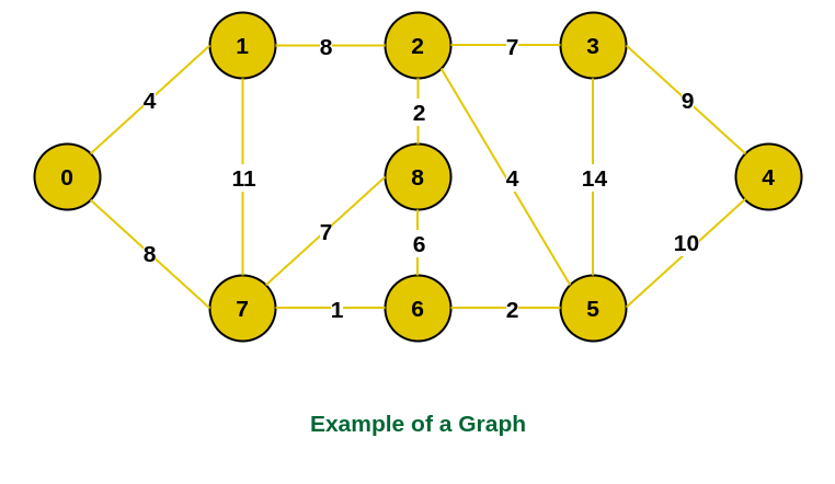
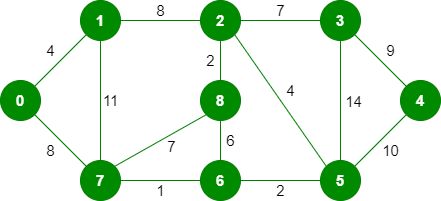
Example of a graph

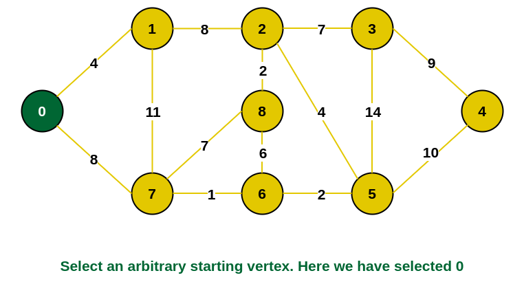
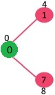
Step 1: Firstly, we select an arbitrary vertex that acts as the starting vertex of the Minimum Spanning Tree. Here we have selected vertex 0 as the starting vertex.

0 is selected as starting vertex

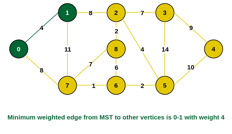
Step 2: All the edges connecting the incomplete MST and other vertices are the edges {0, 1} and {0, 7}. Between these two the edge with minimum weight is {0, 1}. So include the edge and vertex 1 in the MST.

1 is added to the MST

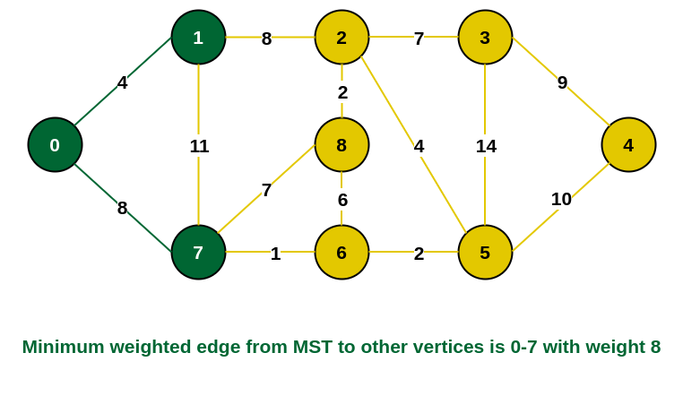
Step 3: The edges connecting the incomplete MST to other vertices are {0, 7}, {1, 7} and {1, 2}. Among these edges the minimum weight is 8 which is of the edges {0, 7} and {1, 2}. Let us here include the edge {0, 7} and the vertex 7 in the MST. [We could have also included edge {1, 2} and vertex 2 in the MST].

7 is added in the MST

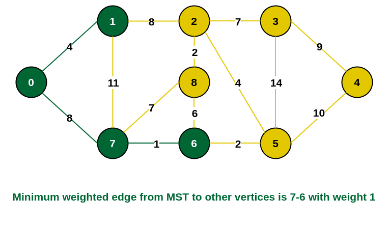
Step 4: The edges that connect the incomplete MST with the fringe vertices are {1, 2}, {7, 6} and {7, 8}. Add the edge {7, 6} and the vertex 6 in the MST as it has the least weight (i.e., 1).

6 is added in the MST

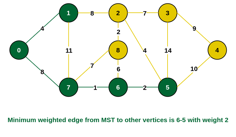
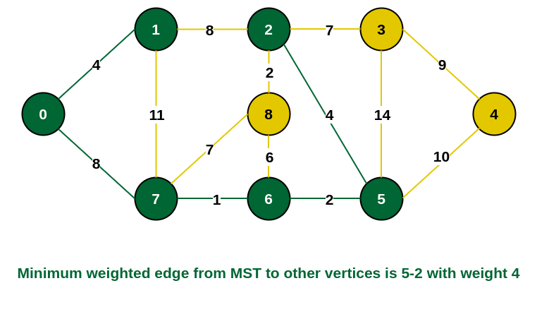
Step 5: The connecting edges now are {7, 8}, {1, 2}, {6, 8} and {6, 5}. Include edge {6, 5} and vertex 5 in the MST as the edge has the minimum weight (i.e., 2) among them.

Include vertex 5 in the MST

Step 6: Among the current connecting edges, the edge {5, 2} has the minimum weight. So include that edge and the vertex 2 in the MST.

Include vertex 2 in the MST

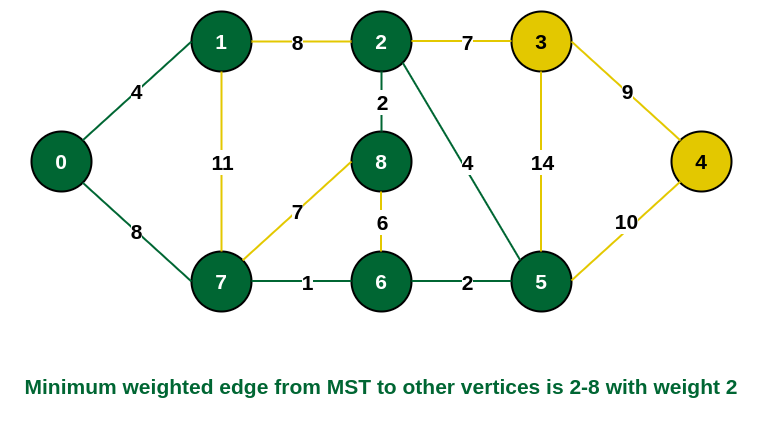
Step 7: The connecting edges between the incomplete MST and the other edges are {2, 8}, {2, 3}, {5, 3} and {5, 4}. The edge with minimum weight is edge {2, 8} which has weight 2. So include this edge and the vertex 8 in the MST.

Add vertex 8 in the MST

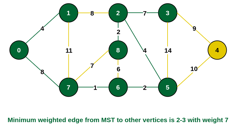
Step 8: See here that the edges {7, 8} and {2, 3} both have same weight which are minimum. But 7 is already part of MST. So we will consider the edge {2, 3} and include that edge and vertex 3 in the MST.

Include vertex 3 in MST

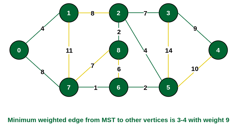
Step 9: Only the vertex 4 remains to be included. The minimum weighted edge from the incomplete MST to 4 is {3, 4}.

Include vertex 4 in the MST

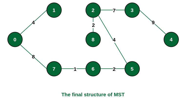
The final structure of the MST is as follows and the weight of the edges of the MST is (4 + 8 + 1 + 2 + 4 + 2 + 7 + 9) = 37.

The structure of the MST formed using the above method

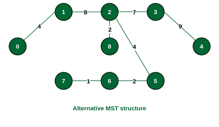
Note: If we had selected the edge {1, 2} in the third step then the MST would look like the following.

Structure of the alternate MST if we had selected edge {1, 2} in the MST

Kruskal’s Algorithm:

1. Sort all the edges in non-decreasing order of their weight.

2. Pick the smallest edge. Check if it forms a cycle with the spanning tree formed so far. If the cycle is not formed, include this edge. Else, discard it.

3. Repeat step#2 until there are (V-1) edges in the spanning tree.

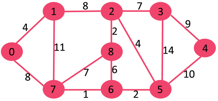
Input Graph:

The graph contains 9 vertices and 14 edges. So, the minimum spanning tree formed will be having (9 – 1) = 8 edges.
After sorting:

Weight	Source	Destination
1	7	6
2	8	2
2	6	5
4	0	1
4	2	5
6	8	6
7	2	3
7	7	8
8	0	7
8	1	2
9	3	4
10	5	4
11	1	7
14	3	5

Now pick all edges one by one from the sorted list of edges

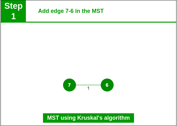
Step 1: Pick edge 7-6. No cycle is formed, include it.

Add edge 7-6 in the MST

Step 2: Pick edge 8-2. No cycle is formed, include it.

Add edge 8-2 in the MST

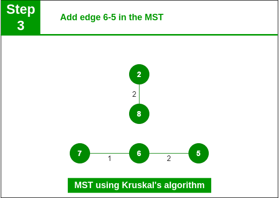
Step 3: Pick edge 6-5. No cycle is formed, include it.

Add edge 6-5 in the MST

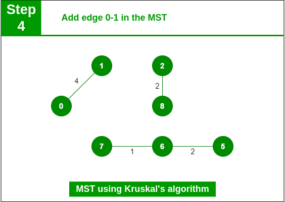
Step 4: Pick edge 0-1. No cycle is formed, include it.

Add edge 0-1 in the MST

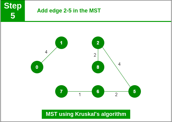
Step 5: Pick edge 2-5. No cycle is formed, include it.

Add edge 2-5 in the MST

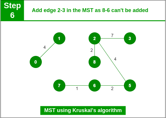
Step 6: Pick edge 8-6. Since including this edge results in the cycle, discard it. Pick edge 2-3: No cycle is formed, include it.

Add edge 2-3 in the MST

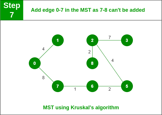
Step 7: Pick edge 7-8. Since including this edge results in the cycle, discard it. Pick edge 0-7. No cycle is formed, include it.

Add edge 0-7 in MST

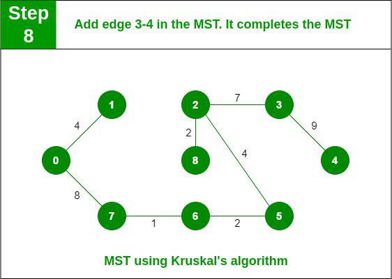
Step 8: Pick edge 1-2. Since including this edge results in the cycle, discard it. Pick edge 3-4. No cycle is formed, include it.

Add edge 3-4 in the MST

Note: Since the number of edges included in the MST equals to (V – 1), so the algorithm stops here

Dijkstra Algorithm:

To understand the Dijkstra’s Algorithm lets take a graph and find the shortest path from source to all nodes.
Consider below graph and src = 0

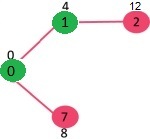
Step 1:

• The set sptSet is initially empty and distances assigned to vertices are {0, INF, INF, INF, INF, INF, INF, INF} where INF indicates infinite.
• Now pick the vertex with a minimum distance value. The vertex 0 is picked, include it in sptSet. So sptSet becomes {0}. After including 0 to sptSet, update distance values of its adjacent vertices.
• Adjacent vertices of 0 are 1 and 7. The distance values of 1 and 7 are updated as 4 and 8.

The following subgraph shows vertices and their distance values, only the vertices with finite distance values are shown. The vertices included in SPT are shown in green colour.

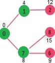
Step 2:

• Pick the vertex with minimum distance value and not already included in SPT (not in sptSET). The vertex 1 is picked and added to sptSet.
• So sptSet now becomes {0, 1}. Update the distance values of adjacent vertices of 1.
• The distance value of vertex 2 becomes 12.

Step 3:

• Pick the vertex with minimum distance value and not already included in SPT (not in sptSET). Vertex 7 is picked. So sptSet now becomes {0, 1, 7}.
• Update the distance values of adjacent vertices of 7( only 7, no vertex 2). The distance value of vertex 6 and 8 becomes finite (15 and 9 respectively).

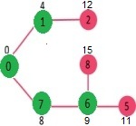
Step 4:

• Pick the vertex with minimum distance value and not already included in SPT (not in sptSET). Vertex 6 is picked. So sptSet now becomes {0, 1, 7, 6}.
• Update the distance values of adjacent vertices of 6. The distance value of vertex 5 and 8 are updated.

We repeat the above steps until sptSet includes all vertices of the given graph. Finally, we get the following Shortest Path Tree (SPT).

Bellman–Ford Algorithm

Step 1: Let the given source vertex be 0. Initialize all distances as infinite, except the distance to the source itself. Total number of vertices in the graph is 5, so all edges must be processed 4 times.

Step 2: Let all edges are processed in the following order: (B, E), (D, B), (B, D), (A, B), (A, C), (D, C), (B, C), (E, D). We get the following distances when all edges are processed the first time. The first row shows initial distances. The second row shows distances when edges (B, E), (D, B), (B, D) and (A, B) are processed. The third row shows distances when (A, C) is processed. The fourth row shows when (D, C), (B, C) and (E, D) are processed.

Step 3: The first iteration guarantees to give all shortest paths which are at most 1 edge long. We get the following distances when all edges are processed second time (The last row shows final values).

Step 4: The second iteration guarantees to give all shortest paths which are at most 2 edges long. The algorithm processes all edges 2 more times. The distances are minimized after the second iteration, so third and fourth iterations don’t update the distances.

Floyd-Warshall Algorithm