
Sorting Algorithm 🌺
1. Merge Sort
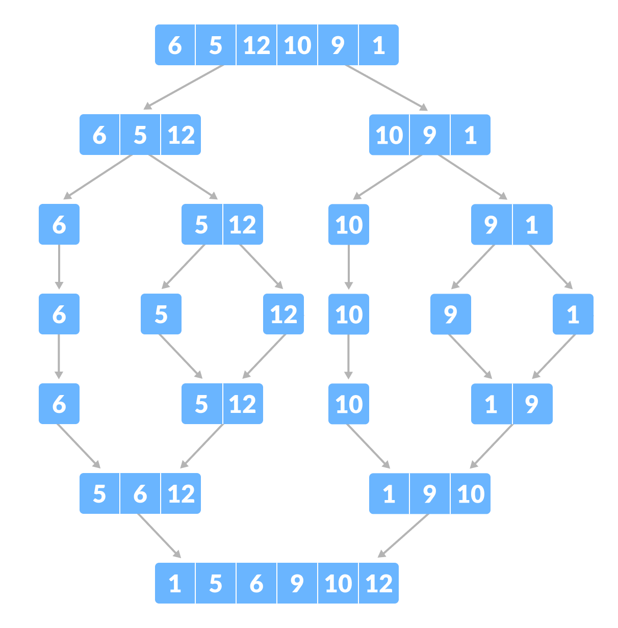
The MergeSort function repeatedly divides the array into two halves until we reach a stage where we try to perform MergeSort on a subarray of size 1 i.e. p == r.
After that, the merge function comes into play and combines the sorted arrays into larger arrays until the whole array is merged.
Pseudocode:
1 | MergeSort(A, p, r): |
JAVA:
1 | // Merge two subarrays L and M into arr |
Merge( ) Function Explained Step-By-Step
Merging two consecutive subarrays of array
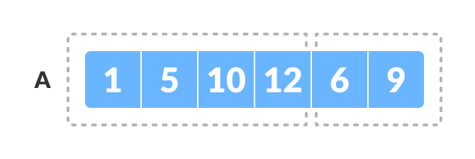
The array A[0..5] contains two sorted subarrays A[0..3] and A[4..5]. Let us see how the merge function will merge the two arrays.
Step 2: Maintain current index of sub-arrays and main array
1 | int i, j, k; |
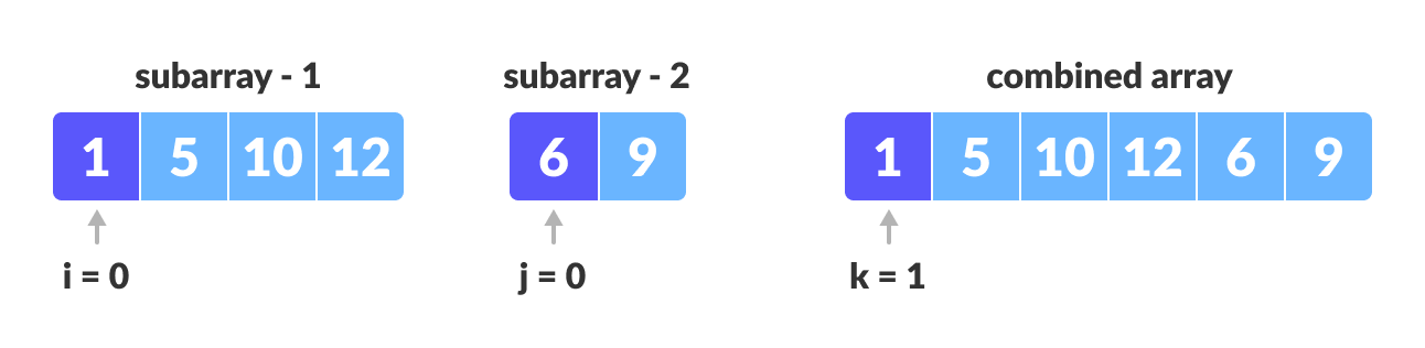 Maintain indices of copies of sub array and main array
Step 3: Until we reach the end of either L or M, pick larger among elements L and M and place them in the correct position at A[p..r]
1 | while (i < n1 && j < n2) { |
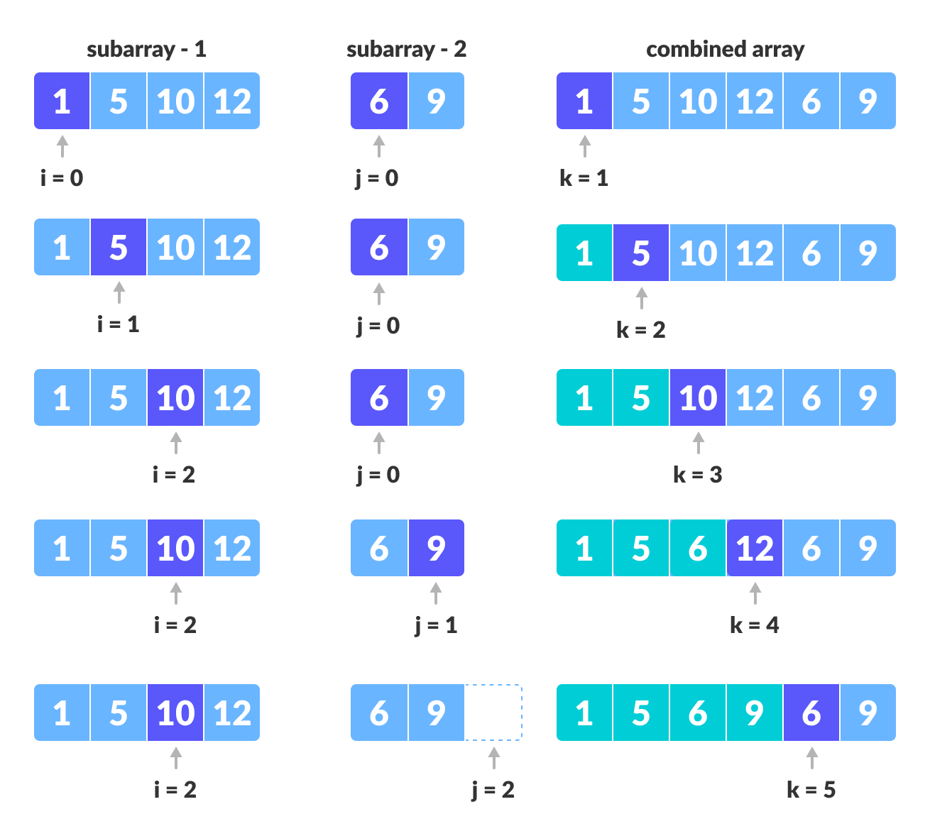 Comparing individual elements of sorted subarrays until we reach end of one
Step 4: When we run out of elements in either L or M, pick up the remaining elements and put in A[p..r]
1 | // We exited the earlier loop because j < n2 doesn't hold |
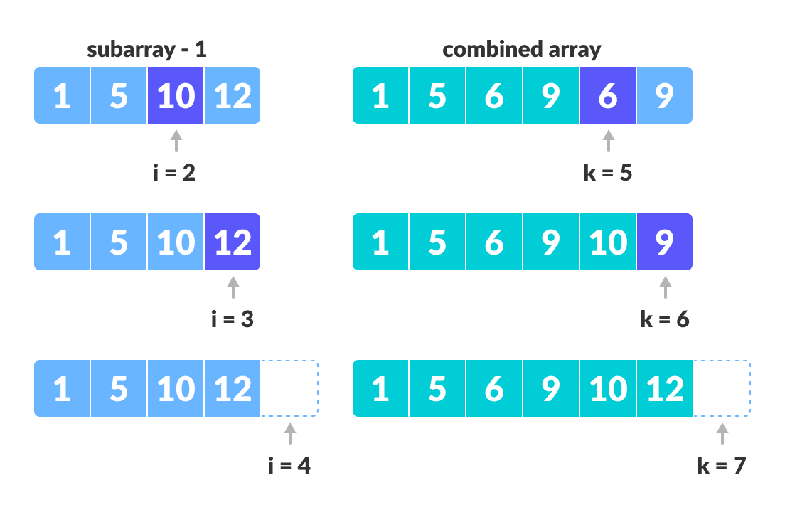 Copy the remaining elements from the first array to main subarray
1 | // We exited the earlier loop because i < n1 doesn't hold |
2. Quick Sort
1. Select the Pivot Element
There are different variations of quicksort where the pivot element is selected from different positions. Here, we will be selecting the rightmost element of the array as the pivot element.
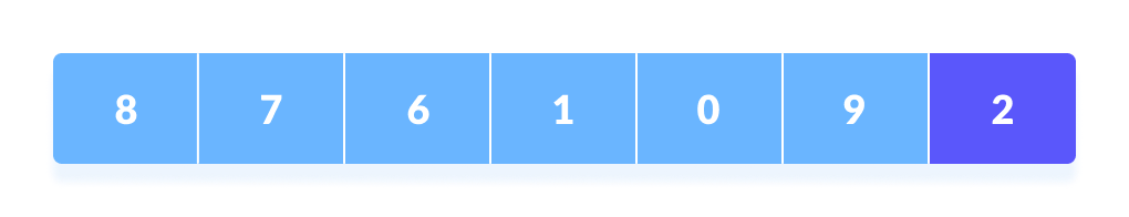 Select a pivot element
2. Rearrange the Array
Now the elements of the array are rearranged so that elements that are smaller than the pivot are put on the left and the elements greater than the pivot are put on the right.
Here’s how we rearrange the array:
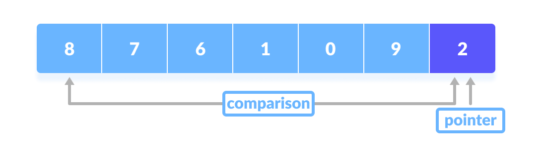
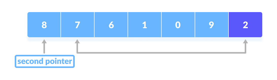
A pointer is fixed at the pivot element. The pivot element is compared with the elements beginning from the first index.

If the element is greater than the pivot element, a second pointer is set for that element.
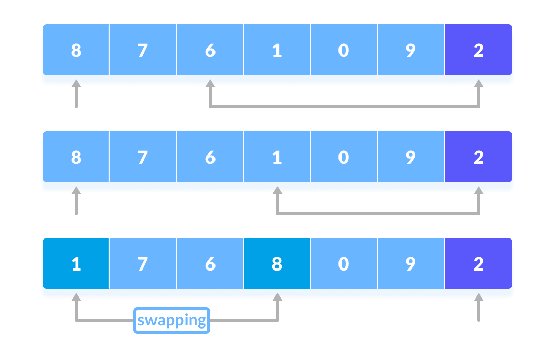
Now, pivot is compared with other elements. If an element smaller than the pivot element is reached, the smaller element is swapped with the greater element found earlier.
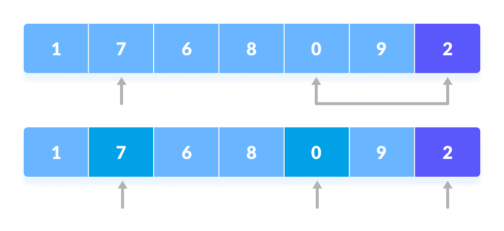
Again, the process is repeated to set the next greater element as the second pointer. And, swap it with another smaller element.
The process goes on until the second last element is reached.
The process goes on until the second last element is reached.Finally, the pivot element is swapped with the second pointer.
Finally, the pivot element is swapped with the second pointer.
 The process goes on until the second last element is reached.
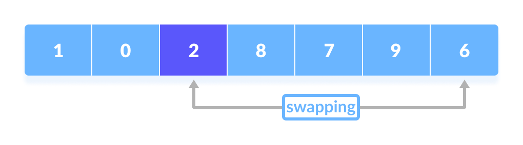 Finally, the pivot element is swapped with the second pointer.
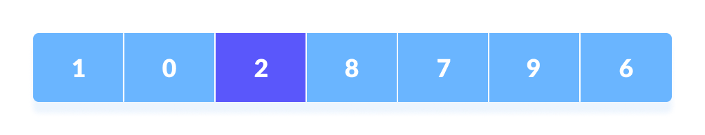
3. Divide Subarrays
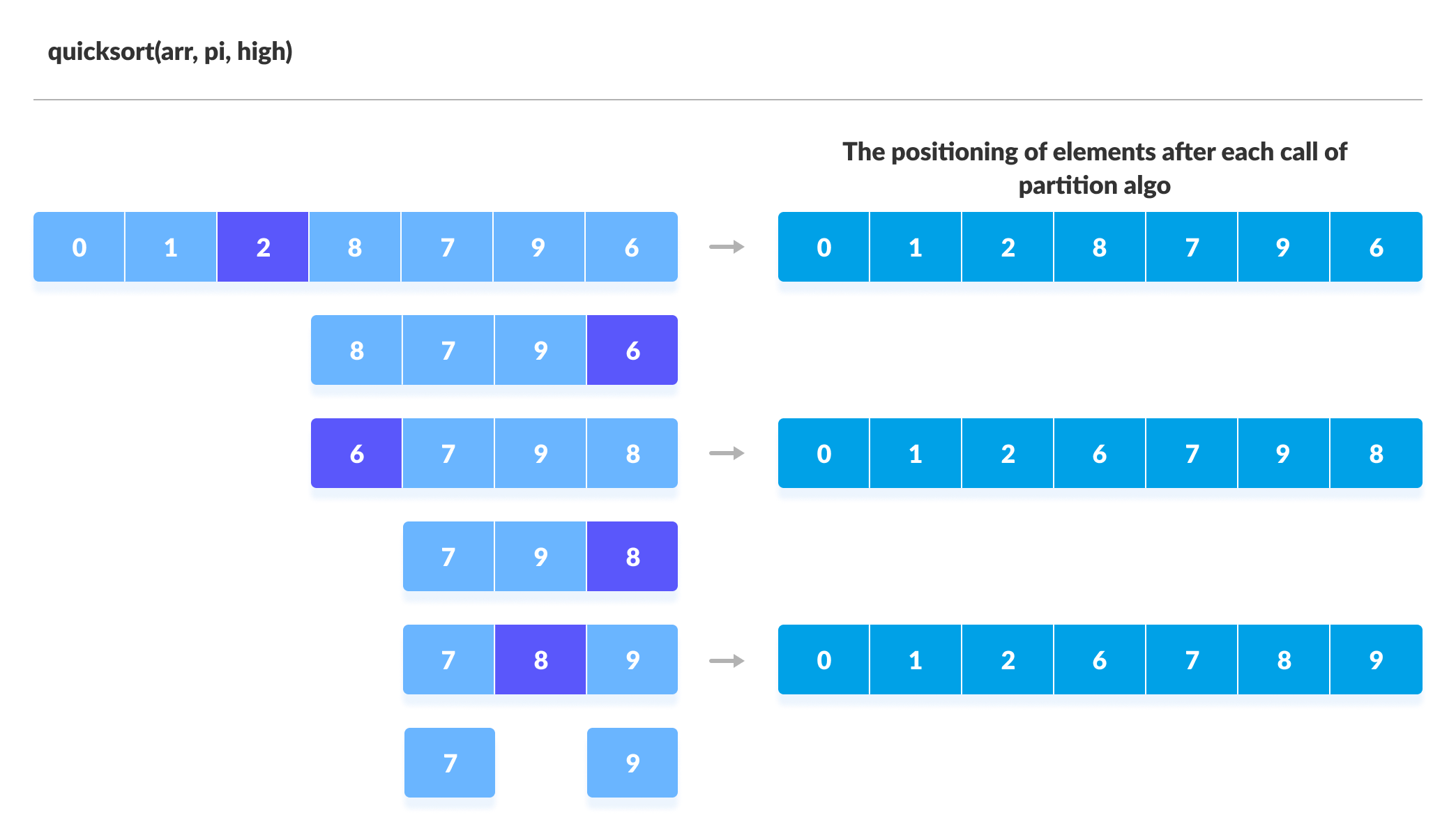
Pivot elements are again chosen for the left and the right sub-parts separately. And, step 2 is repeated.
pseudocode
1 | quickSort(array, p, r) |
JAVA
1 | // Quick sort in Java |
3.Counting Sort
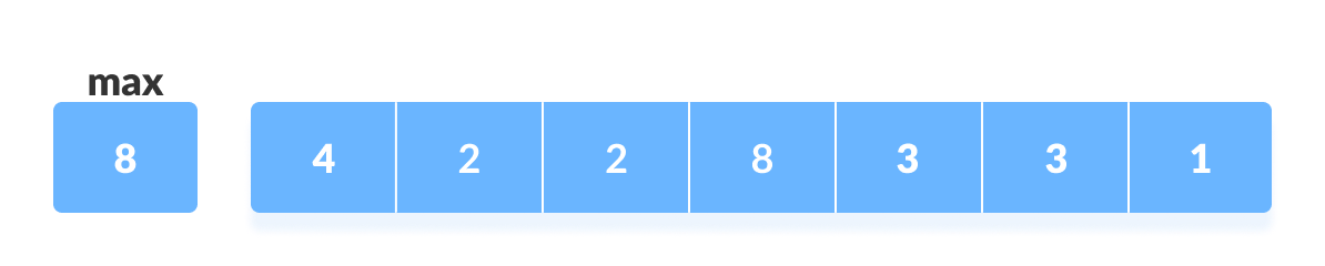
- Find out the maximum element (let it be
max) from the given array.
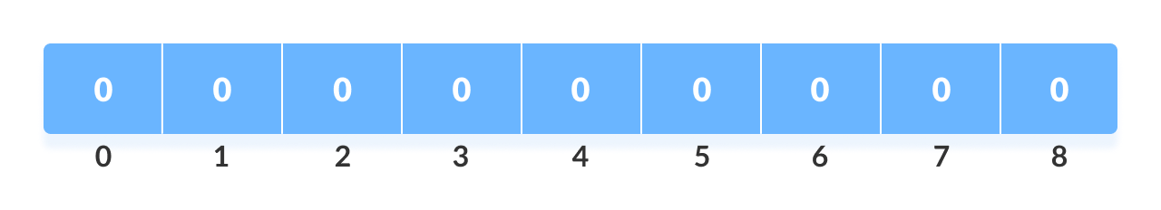
- Initialize an array of length
max+1with all elements 0. This array is used for storing the count of the elements in the array.
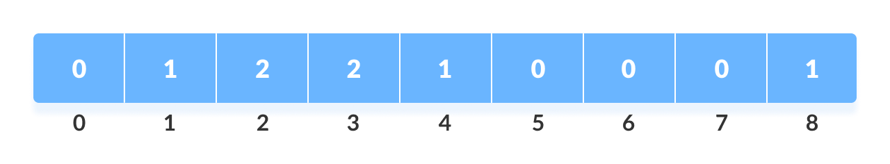
- Store the count of each element at their respective index in
countarray
For example: if the count of element 3 is 2 then, 2 is stored in the 3rd position of count array. If element “5” is not present in the array, then 0 is stored in 5th position.
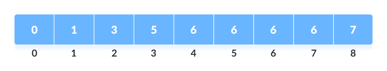
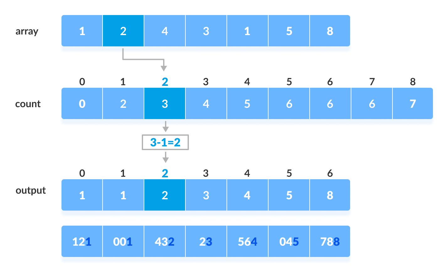
4. Store cumulative sum of the elements of the count array. It helps in placing the elements into the correct index of the sorted array. (0, 0+1, 0+1+2, 0+1+2+2…..)
- Find the index of each element of the original array in the count array. This gives the cumulative count. Place the element at the index calculated as shown in figure below.
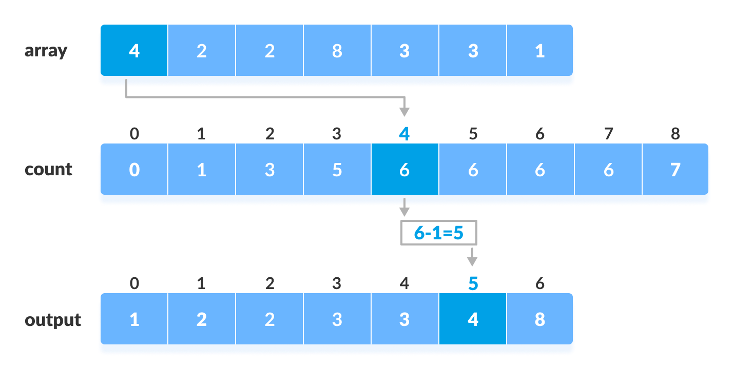 6. After placing each element at its correct position, decrease its count by one.
Pesudocode
1 | countingSort(array, size) |
JAVA
1 | // Counting sort in Java programming |
4. Bucket Sort
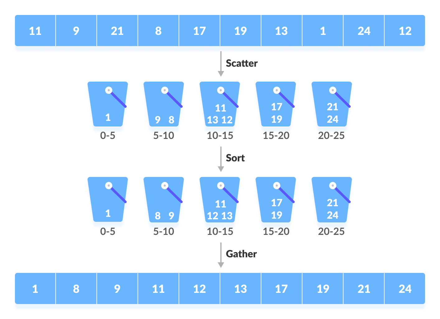
The process of bucket sort can be understood as a scatter-gather approach. Here, elements are first scattered into buckets then the elements in each bucket are sorted. Finally, the elements are gathered in order.
!!!!!!!
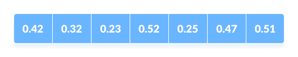
Suppose, the input array is:
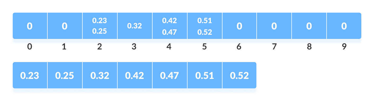
Input arrayCreate an array of size 10. Each slot of this array is used as a bucket for storing elements.
Array in which each position is a bucketInsert elements into the buckets from the array. The elements are inserted according to the range of the bucket.
In our example code, we have buckets each of ranges from 0 to 1, 1 to 2, 2 to 3,…… (n-1) to n.
Suppose, an input element is 0.23 is taken. It is multiplied by size = 10 (ie. 0.23*10=2.3 ). Then, it is converted into an integer (ie. 2.3≈2 ). Finally, .23 is inserted into bucket-2.
Similarly, 0.25 is also inserted into the same bucket. Everytime, the floor value of the floating point number is taken.
If we take integer numbers as input, we have to divide it by the interval (10 here) to get the floor value.
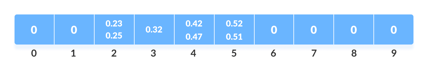
Similarly, other elements are inserted into their respective buckets.
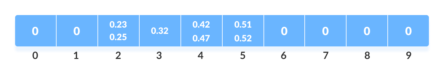
The elements of each bucket are sorted using any of the stable sorting algorithms. Here, we have used quicksort (inbuilt function).
The elements from each bucket are gathered.
It is done by iterating through the bucket and inserting an individual element into the original array in each cycle. The element from the bucket is erased once it is copied into the original array.
 Input array
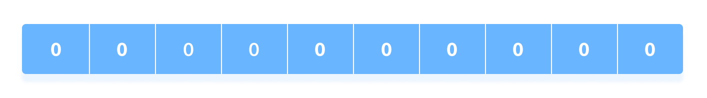 Array in which each position is a bucket
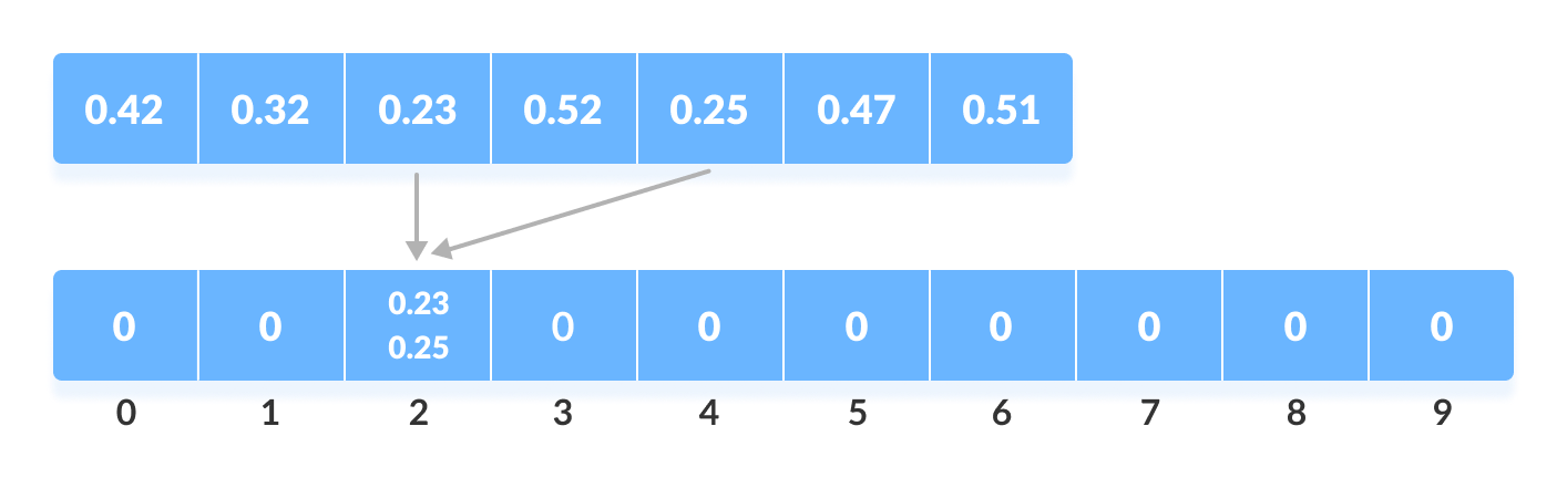
Bucket sort is used when:
- input is uniformly distributed over a range.
- there are floating point values
Pseudocode
1 | bucketSort() |
Java
1 | // Bucket sort in Java |
Radix Sort
Find the largest element in the array, i.e. max. Let
Xbe the number of digits inmax.Xis calculated because we have to go through all the significant places of all elements.In this array
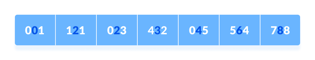
[121, 432, 564, 23, 1, 45, 788], we have the largest number 788. It has 3 digits. Therefore, the loop should go up to hundreds place (3 times).Now, go through each significant place one by one.
Use any stable sorting technique to sort the digits at each significant place. We have used counting sort for this.
Sort the elements based on the unit place digits (X=0).
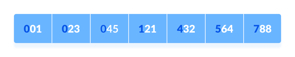
Now, sort the elements based on digits at tens place.
Finally, sort the elements based on the digits at hundreds place.
Pseudocode
1 | radixSort(array) |
Java
1 | // Radix Sort in Java Programming |
5. Heap Sort
Detailed Working of Heap Sort
To understand heap sort more clearly, let’s take an unsorted array and try to sort it using heap sort.
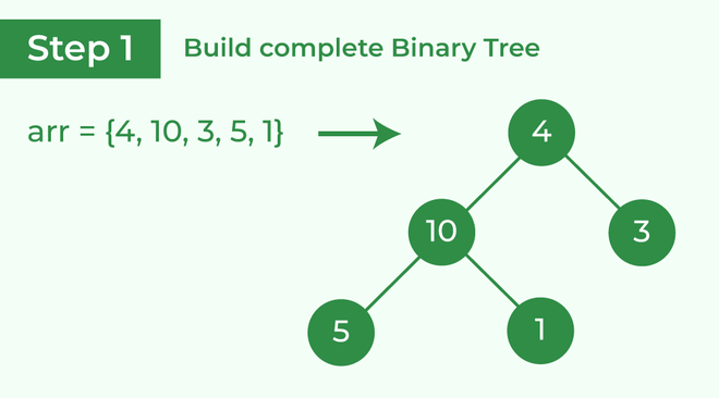
Consider the array: arr[] = {4, 10, 3, 5, 1}.Build Complete Binary Tree: Build a complete binary tree from the array.
Build complete binary tree from the array
Transform into max heap: After that, the task is to construct a tree from that unsorted array and try to convert it into max heap.
- To transform a heap into a max-heap, the parent node should always be greater than or equal to the child nodes
- Here, in this example, as the parent node 4 is smaller than the child node 10, thus, swap them to build a max-heap.
Transform it into a max heap image widget
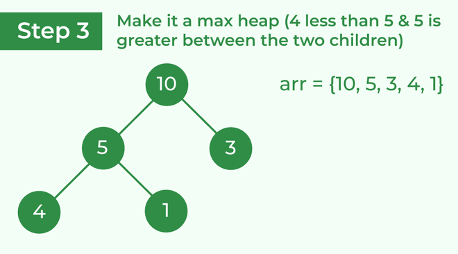
- Now, as seen, 4 as a parent is smaller than the child 5, thus swap both of these again and the resulted heap and array should be like this:
Make the tree a max heap
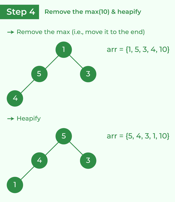
Perform heap sort: Remove the maximum element in each step (i.e., move it to the end position and remove that) and then consider the remaining elements and transform it into a max heap.
- Delete the root element from the max heap. In order to delete this node, try to swap it with the last node, i.e. After removing the root element, again heapify it to convert it into max heap.
- Resulted heap and array should look like this:
Remove 10 and perform heapify
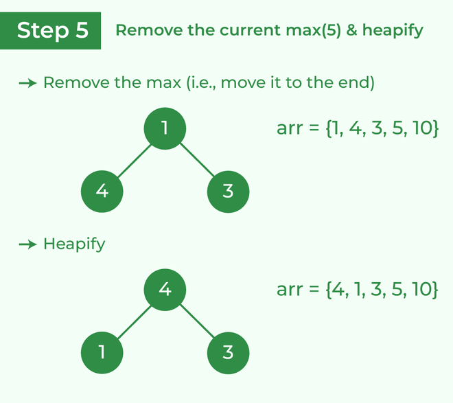
- Repeat the above steps and it will look like the following:
Remove 5 and perform heapify
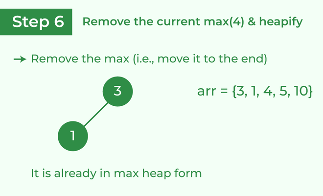
- Now remove the root (i.e. 3) again and perform heapify.
Remove 4 and perform heapify
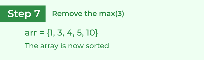
- Now when the root is removed once again it is sorted. and the sorted array will be like arr[] = {1, 3, 4, 5, 10}.
Complexity
Quicksort Complexity
| Time Complexity | |
|---|---|
| Best | O(n*log n) |
| Worst | O(n2) |
| Average | O(n*log n) |
| Space Complexity | O(log n) |
| Stability | No |
Worst Case Complexity [Big-O]:
O(n2)
It occurs when the pivot element picked is either the greatest or the smallest element.This condition leads to the case in which the pivot element lies in an extreme end of the sorted array. One sub-array is always empty and another sub-array contains
n - 1elements. Thus, quicksort is called only on this sub-array.However, the quicksort algorithm has better performance for scattered pivots.
Best Case Complexity [Big-omega]:
O(n*log n)
It occurs when the pivot element is always the middle element or near to the middle element.Average Case Complexity [Big-theta]:
O(n*log n)
It occurs when the above conditions do not occur.
Merge Sort Complexity
| Time Complexity | |
|---|---|
| Best | O(n*log n) |
| Worst | O(n*log n) |
| Average | O(n*log n) |
| Space Complexity | O(n) |
| Stability | Yes |
Counting Sort Complexity
| Time Complexity | |
|---|---|
| Best | O(n+k) |
| Worst | O(n+k) |
| Average | O(n+k) |
| Space Complexity | O(max) |
| Stability | Yes |
Time Complexities
There are mainly four main loops. (Finding the greatest value can be done outside the function.)
| for-loop | time of counting |
|---|---|
| 1st | O(max) |
| 2nd | O(size) |
| 3rd | O(max) |
| 4th | O(size) |
Overall complexity = O(max)+O(size)+O(max)+O(size) = O(max+size) max -> n, size->k
- Worst Case Complexity:
O(n+k) - Best Case Complexity:
O(n+k) - Average Case Complexity:
O(n+k)
In all the above cases, the complexity is the same because no matter how the elements are placed in the array, the algorithm goes through n+k times.
The space complexity of Counting Sort is O(max). Larger the range of elements, larger is the space complexity.
Bucket Sort Complexity
| Time Complexity | |
|---|---|
| Best | O(n+k) |
| Worst | O(n2) |
| Average | O(n) |
| Space Complexity | O(n+k) |
| Stability | Yes |
- Worst Case Complexity:
O(n2)
When there are elements of close range in the array, they are likely to be placed in the same bucket. This may result in some buckets having more number of elements than others.
It makes the complexity depend on the sorting algorithm used to sort the elements of the bucket.
The complexity becomes even worse when the elements are in reverse order. If insertion sort is used to sort elements of the bucket, then the time complexity becomesO(n2). - Best Case Complexity:
O(n+k)
It occurs when the elements are uniformly distributed in the buckets with a nearly equal number of elements in each bucket.
The complexity becomes even better if the elements inside the buckets are already sorted.
If insertion sort is used to sort elements of a bucket then the overall complexity in the best case will be linear ie.O(n+k).O(n)is the complexity for making the buckets andO(k)is the complexity for sorting the elements of the bucket using algorithms having linear time complexity at the best case. - Average Case Complexity:
O(n)
It occurs when the elements are distributed randomly in the array. Even if the elements are not distributed uniformly, bucket sort runs in linear time. It holds true until the sum of the squares of the bucket sizes is linear in the total number of elements.
Radix Sort Complexity
| Time Complexity | |
|---|---|
| Best | O(n+k) |
| Worst | O(n+k) |
| Average | O(n+k) |
| Space Complexity | O(max) |
| Stability | Yes |
Since radix sort is a non-comparative algorithm, it has advantages over comparative sorting algorithms.
For the radix sort that uses counting sort as an intermediate stable sort, the time complexity is O(d(n+k)).
Thus, radix sort has linear time complexity which is better than O(nlog n) of comparative sorting algorithms.
If we take very large digit numbers or the number of other bases like 32-bit and 64-bit numbers then it can perform in linear time however the intermediate sort takes large space.
This makes radix sort space inefficient. This is the reason why this sort is not used in software libraries.
[TOC]